Update 12/12/2021
Since writing this post in 2017, Excel now has new revolutionary dynamic array formulas that really has overtaken all the workarounds for better dropdown lists we used to do such as described in my post below. Now the new formula SORT() + UNIQUE() in Excel Office 365 (although not in earlier stand alone Excel versions) is simply the best way of returning a sorted dropdown list.
A quick demo on how…say your list data is in A2:A10 then
- in say C1 create your list enter = SORT(UNIQUE(A2:A10)) which gives you a dynamic array list of no blanks in between items and sorted.
- where you want your dropdown say H1 in the data validation dialog source field enter =C1#
That’s it. So much easier to implement than it used to be.
But better to place the dropdown list within a Table which is dynamic. Briefly how – convert the A2:A10 list to a Table (from a cell within this range Control T, My Table has headers unticked) change the column name to ‘MyList’ and change the name of the Table in the ribbon context Menu ‘Table Design’ to MyTable. Then change the range reference in C1 from A2:A10 to MyTable[Mylist] . Any new items to your table column list will be included because the dropdown in H1’s validation source field is pointing to a dynamic array list in C1 which in turn has a formula pointing to your new inherently dynamic ‘MyTable’ Table column, ‘MyList’.
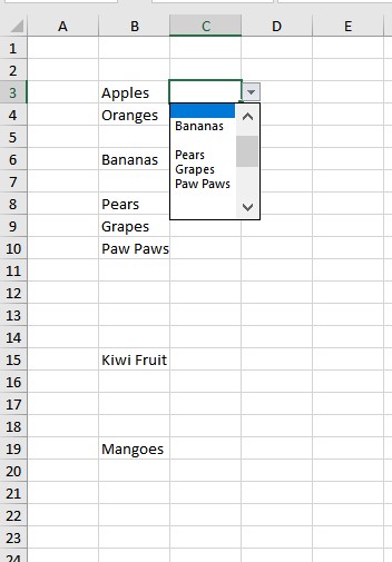
For a dependent dropdown, you can use SORT() + UNIQUE() + FILTER() – see this nice short and sweet 3 min video from Bill Jelen Mr Excel https://www.youtube.com/watch?v=3eLzIMGpi5g on how.
I am leaving the post below to help people with older Excel versions.
Published Sep 10, 2017
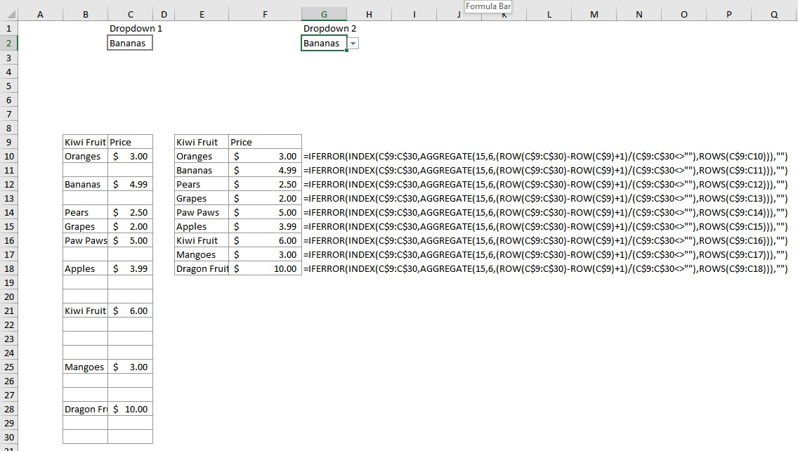
Sometimes you just need to get rid of the gaps in lists! Perhaps you want to use the list for a validation dropdown and you want no gaps in the list so it’s easier to use. Perhaps you just want to create a better looking table from a long list of values.
I use this formula all the time for these situations, so it’s a good one to have in your Excel tool kit ready to use.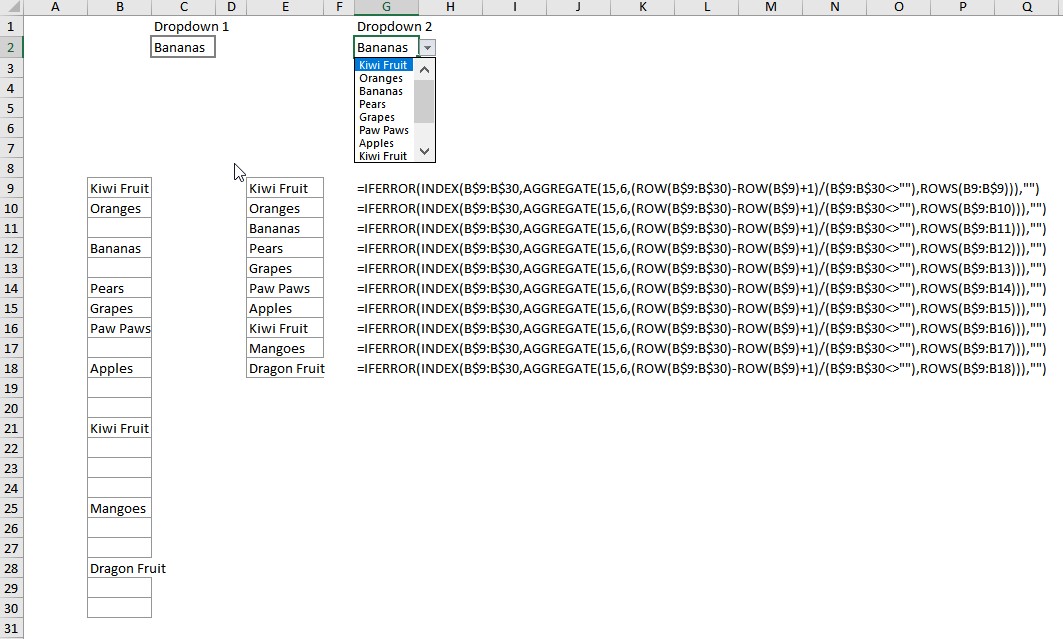
=IFERROR(INDEX(B$9:B$30,AGGREGATE(15,6,(ROW(B$9:B$30)-ROW(B$9)+1)/(B$9:B$30<>””),ROWS(B9:B$9))),””)
Note carefully where the anchoring is row being the start of the list in column B, row 30 being the end including some spaces. The formula is copied down until all the items in B appear in the new list. in column E.
But there are situations where you have many rows of data and formulas on each row highlighting or extracting something but you need to neatly summarise. Well the above formula is ready to be dragged across to pick up the next columns data and so on.