I have blogged before about how much I love INDEX (INDEX what’s the Big Deal ). It’s powerful, nimble (non volatile so easy on performance load) and just makes so much sense to me given we are working with a grid and INDEX essentially returns the contents from the co-ordinates of the grid reference entered. Essentially in English INDEX returns the contents of this ROW and this COLUMN for this array (or range). We then can get smart about which Row and which column using MATCH or other formulas we can use with criteria. So don’t forget to think about using INDEX wrapped within other formulas like SUM to give you a dynamic summing solution. Both ends of the SUM formula can have an INDEX formula so you can have a dynamic start and end to your SUM range. In the following real world example we will have an INDEX formula as the start of our SUM range to a static end of the SUM range (C3).
Take for example a situation like below where you have a list of actuals by month (I haven’t bothered to show the months) and you want to compare against meaningful averages. A good analyst won’t want to just statically report against say a fixed 12 months. He or she knows that recent events may mean comparing to the last quarter is more revealing because there has been say a sustained growth in business level and a quarterly average is more important than an annual average. Or they might just know their boss might ask for anything so why not build the formula flexible enough for any average!
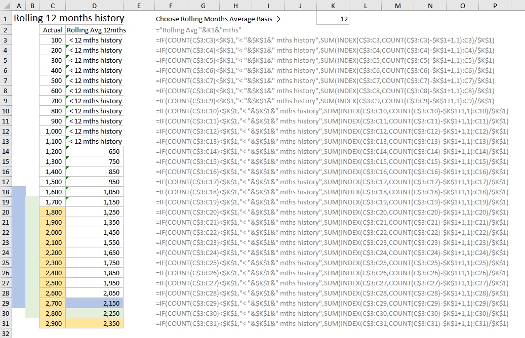
So in the below example K1 has a cell to set the rolling average period in months to be used. The formulas then in D3:D31 show a calculation for an average based on what the user enters in K1
=IF(COUNT(C$3:C3)<$K$1,”< “&$K$1&” mths history”,SUM(INDEX(C$3:C3,COUNT(C$3:C3)-$K$1+1,1):C3)/$K$1)
So this part of the formula SUM(INDEX(C$3:C3,COUNT(C$3:C3)-$K$1+1,1):C3)/$K$1) uses SUM to dynamically figure out where is the cell positioned in the list and what is the SUM of this cell back X prior months (to the number chosen by the user in k1), then its simple averaged.
The first part of the formula IF(COUNT(C$3:C3)<$K$1,”< “&$K$1&” mths history”, is simply handling the fact that once you go back to the beginning of a list you can run out of cells to use in the average. You might handle this differently and allow an average for less months than chosen by the use in K1 where the formula runs out of data.
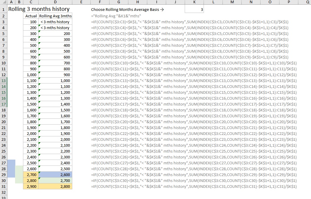 But if you want 12 months it’s just a matter of entering this to K1 instead.