
So back to my scenario, yes you could copy, then paste special, transpose values only. Yes I could use Power Query that’s true and probably will as my long term solution. But hey I am a data analyst and anything I do even quick fixes, I am going to automate in case I have to do it again. Automate or die should be one of your mantras.
 So I get cracking – I add a data validation in G4 of the date column so I can have a dynamic starting point. If you were pushed for time G4 could just simply have 01/07/17 entered directly. I went the data validation route because next time my Accountant boss might want a report with 2 year’ s sales on a calendar year basis so I can easily choose another starting point in the validation drop down. With this starting date to my data set, we can use formulas to give us the dates we want using DATE function and then our INDEX formula can use these dates to to go and get the sales pertaining to the dates I want. Now I am assuming we want to report consecutive months in this type of report. So to get the months to increment by 1 across the page – I use the relative DATE formula in H4 =DATE(YEAR(G4),MONTH(G4)+1,DAY(G4)) – basically I am leaving the YEAR and DAY alone but incrementing the MONTH by one. Copy this across and of course the it will increment by 1 month. Now I use my INDEX / MATCH combo formula:
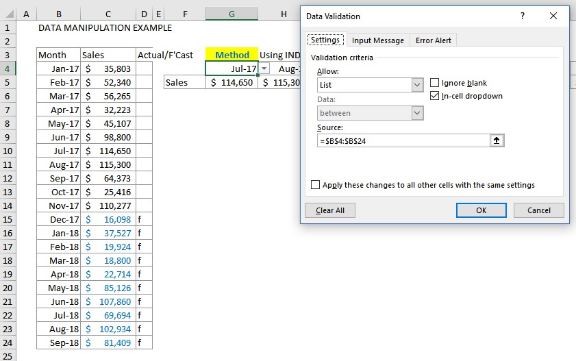
=INDEX($B$4:$C$24,MATCH(G4,$B$4:$B$24,0),2) and it uses the date in G4 in the MATCH function within the vector $B$4:$B$24
to return the position of the date and then return the corresponding value from the 2nd column within the array $B$4:$C$24 defined in the first part of the function. You could give the array and vector range names if you want. Also would make the array $B$4:$C$24 a n Excel Table so it’s dynamic for future data. Anyway this is a simple example – copied across the formula effortlessly returns the corresponding date’s sales.
