This a post about a handy little formula I came up with on a job last week in order to test formulas from a client’s solution, against a list of specific ‘newish’ Microsoft 365 formulas like LAMBDA() and TOCOL() not present in his version. I needed to replace these formulas with older formulas.

How I got the list of formulas in itself is another interesting story which I will detail at the end.

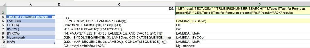
So this formula as above in D 5:D10 detailed in D3, uses SEARCH() to look up the Table in A 4 (Table 1) for the text of the formulas that I am testing for in the list of made up formulas in column C below. It returns multiple matches of the text from Table 1 separated by comma. The fact that it handles multiple matches and they are listed in the result makes this a not so common formula (I couldn’t find anything similar after googling for quite a while) so by no means am I claiming it to be the first, but I was pretty pleased to come up with it to solve my real world problem and now share.

Dissecting this formula a little…

- the LET aspect is not so critically important in this formula as the calculation part was only needed twice in the formula but it makes it that bit tidier and more readable
- the SEARCH formula (which is not case sensitive unlike its sister formula FIND) works with wildcards critical to this problem. You might want case sensitivity, in which case change to FIND from SEARCH.
- ISNUMBER creates TRUE / FALSE outcomes for the Table 1 list of possible matches within that cell.

These TRUES and FALSEs allow the IF part of the formula to return the match itself or an “OK” and then TEXTJOIN, a dynamic array formula, collects it all together.

So the other part of this story is the LAMBDA formula you can use to list or documents formulas in a given range as shown in Col C above. Huge thanks to Mike Girvan for this tool from his awesome You Tube video (awesome being a superlative that doesn’t really do it justice) on the Excel LAMBDA function – “Every Single Thing You Ever Wanted To Know – 365 MECS 10” . Now amongst so many other scarcely believable feats in this video, Mike has a immensely useful ‘day to day’ LAMBDA formula he named SHOWFORMULAS in the Name Manager at about 32:17 in the video. In the worksheet =SHOWFORMULA(FormulaRange) creates a vertical list of formulas for the purpose of documenting / displaying formulas which has been a challenge in the past. The reference in the LAMBDA below is the range of formulas you want to show in the vertical displayed result.

=LAMBDA(
reference,IFERROR(TOCOL(ADDRESS(ROW(reference), COLUMN(reference), 4) & ": " & FORMULATEXT(reference), 2), ""))

Now I had a problem with the IFERROR() part of Mike’s formula and can’t figure out why, but something in my formulas was triggering the IFERROR part of his formula even though my formulas, the target of Mike’s formula, weren’t actually returning errors. So I removed the IFERROR component and it worked great so be aware of this. So my version of Mike’s formula is below…

=LAMBDA(reference,
TOCOL(ADDRESS(ROW(reference),COLUMN(reference),4)&": "&FORMULATEXT(reference),2,FALSE))

If you are not aware of Mike Girvan’s Excel is Fun You Tube channel then let me just say he has 865K subscribers and just 1000s of videos covering all aspects of Excel from beginner to nerd level expert and his teaching content, style and visual delivery is legendary.