

Excel MVPs have helped us all with a ton of videos and posts out there introducing these new functions. Just Google Excel new Dynamic Array formulas and you are away. Here is the full list of new Dynamic Array formulas:
So only a brief recap – these are revolutionary in our Excel world because in the past, formulas fundamentally have been built to return an answer to one cell. They might use ranges or vectors but they were designed to return the result to one cell. These new Dynamic Array formulas can return a variable column or range (called a spill range) of values. That’s really different.
I remember back then I had to make a conscious effort to understand Excel Tables when they were introduced to Excel 2007. The syntax of Table formulas was different (called Structured References) and they have quirks you need to understand such as you can’t have formulas in the Table headings and Headings must be unique. Now, I can’t imagine not using them where ever I can. I have a post on why you need to form the habit of using Tables here.
Similarly, with these Dynamic Array formulas, you need to spend a little time playing with them and getting to understand them so they are on your radar for your day to day work.
So what are they all about. Like Tables, they help make your Excel work more dynamic and interactive. They also mean less resource sapping complex formulas (and often Array formulas) trying to achieve the same things these new formulas now do. Below are some examples exploring UNIQUE, SORT, SORTBY and FILTER (possibly the star of these new formulas for me) to hopefully inspire everyday users to start using these new formulas.
So the following examples refer to this example which you can click on to enlarge and print if you want.
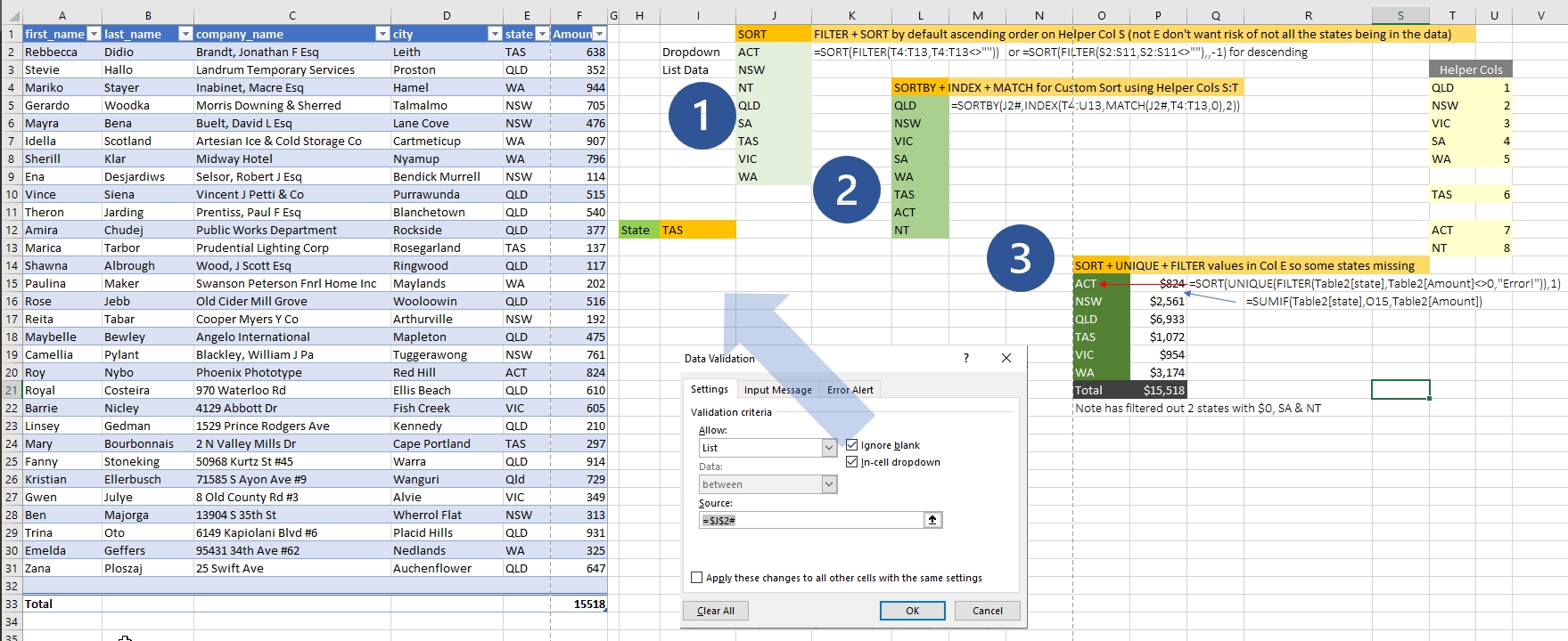
- Dropdown Lists (FILTER + SORT) I am constantly building data validation dropdown lists into my models as I am sure are like lots of people – it ensures reliable data entry where it counts and makes data entry easier for the user. But how many times have you had lists you wanted to use that had duplicate entries or annoying spaces you had to solve with complex workarounds. So in the below No. 1 example J2 =SORT(FILTER(T4:T13,T4:T13<>””)) which is extracting a list from T4:T13 which has (intentional) gaps it is filtering out. So I didn’t use Col E with UNIQUE() for getting my States, as with real data you can’t be sure all the States will be represented in the transactional data, so hence using the Helper range of all possible States. Then in I12 you set up the data validation (on the ribbon Data \ Data Validation \ Allow List with Source = $I$2# . The “#” part of the syntax refers to the spill range that starts in J2 which we want in the dropdown. Note the Helper cell range was just for the example – in real life if I had data like cost codes or product codes I would define them in a Table so dropdown lists are dynamic. Not many new States in Australia lately so this was not realistic in my example.
~ - SORTBY can be used to allow for sorting in a custom way using another range or array order so No2 example below shows how easy it is to have a particular State order. L5 =SORTBY(J2#,INDEX(T4:U13,MATCH(J2#,T4:T13,0),2)) . This has made this Data Validation dropdown feature much more what people have always needed. I have a Civil Engineering client who wants a custom order in their dropdowns reflecting the most commonly used costs codes appearing first. So for me, that’s 2 problems gone that we have always had with these dropdowns 1) gaps and 2) the order. There is 3) getting unique data from ranges but be careful in using UNIQUE for drop downs as it may be missing items at a point in time and you may need to report $0. OK autocomplete is still missing from these dropdowns which actually Goggle Sheets has and we all want in Excel. One day….
~ - Returning Filtered list/range capability within formulas (SORT + UNIQUE + FILTER). Up until now your choice for getting filtered data were copying and pasting from a Pivot Table, Autofilter and Advanced Filter, or using formulas SUMPRODUCT and SUMIFS/SUMIF/COUNTIFS/COUNTIF (I will call these SUMIFS and friends) if summing. The first three of these return filtered lists or ranges but are not formulas and take a little time to set up as an intermediary step and are not live and so need to be refreshed or re-run. The next two SUMPRODUCT and the SUMIFS and friends are great filtering formulas that have served and can still serve us well, but they don’t return to us a filtered list or range and are performance sapping in the case of SUMPRODUCT and SUMIFS and friends cumbersome if you want OR logic.Now we have FILTER and it’s a formula, it can easily do AND or OR logic, that recalculates automatically, can easily slot into our other formulas and return us a list or range of filtered data if we want. That’s a pretty big change! See my example below No.3 in O15 =SORT(UNIQUE(FILTER(Table2[state],Table2[Amount]<>0,”Error!”)),1). This is just a modest use of FILTER but it’s filtering out the States (SA & NT) that have zero dollars in Col F. UNIQUE is taking care of the multiple instances of each state in Col E and then returning us a list sorted in the default Ascending order. We couldn’t do this before in a formula.