
In my recent post of Fix duplicated Conditional Formatting Rules , I mentioned you should be careful using Conditional Formatting in situations where you have thousands of rows of data or calculations as this can be a drain on performance. I also mentioned you can use alternatives in these situations and just thought I would show a simple and silly really illustration as wells as a real world example further below. The following example uses Wingdings / Wingdings2 type coloured fonts but of course it can be just words like “ERROR!” or as one of my recent clients used much to my amusement “WTF!”. The formula in each cell of B4:G9 is the same as that shown in the Formula edit bar varied for each “flag” type that you could use in different columns of a large data set to highlight various conditions you might have.
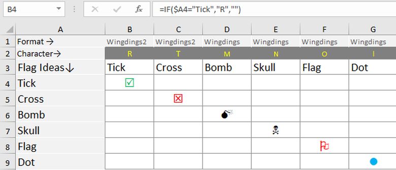 If you can decide on the same font (eg just Wingdings) and colour you can combine to one column and use an IF and OR combination or a CHOOSE formula to test multiple mutually exclusive conditions. I have used Boolean logic here in a CHOOSE formula to keep the example formula simpler and have just done the first 2 possibilities ie =CHOOSE(($A4=”Tick”)*1+($A4=”Cross”)*2,+.. and so on …. ,”R”,”T”… and so on so the formula can only return an index number for which you have a result in the same Font format). Note in my example you couldn’t use the non Wingdings 2 symbols in the same formula and you would have to pick symbols from the same font set. Note also, probably obvious, if you use this Boolean formula structure, the conditions must be mutually exclusive.
So now more practically, say you you want to check for various issues and errors or omissions in manual data entry across a row using say the error Flag in Wingdings. I recently used this formula across columns within a Table to return the text either OVERDUE or <-CHK ENTRY. This text could have just as easily returned a Wingdings Flag and one other symbol instead of the text used.
=IF(AND(A11391<>””,[@[Date Received]]<>””,[@[XX Test No.]]<>”No Testing Required”,O11391=”No Release Date”,NOW()-I11391>90),”OVERDUE”,IF(AND(A11391<>””,COUNTBLANK(C11391:L11391)>1),”<-CHK ENTRY”,””))
I hesitate to use this example because it was borne out of a large legacy spreadsheet situation. Its ignoring the Table header in some formula parts which you shouldn’t do as you can have problems with Tables expanding (as I eventually did see p.s.). But this was a large legacy spreadsheet and I drew a red line at a certain row after which this formula applied and before which I didn’t want any past data from previous legacy formulas to be affected and all this to be within a newly applied Table. The main thing here is it illustrates you can do a number of tests on cells across a row range in one column to highlight issues or errors about the range. In this case it checked if there was a transaction that was overdue first and foremost and if not, then test if there were blanks in C:L.
Don’t get me wrong with this post. Conditional Formatting is great in many situations like dashboards and reports. But good spreadsheet design means maintaining good Excel performance and if you have thousands of rows like in my real world example, using Conditional Formatting would have caused a performance problem especially as there rows are growing with growing data. So in that situation I felt I needed to use a more nibbler alternative. Note my earlier post shows ways to avoid or fix that situation if it’s caused by users in their copying and pasting.
p.s. Yes in my practical real world example sure enough I did have problems with the Table expanding properly due to the formulas not being consistent throughout each Table column. With Tables, the golden rule is Table column rows should have the same formulas and formatting from top to bottom. I solved this with macros to add new Table rows to ensure the new formulas and formats carried on with new lines.